Tabular Reporting with R Markdown

February 9, 2020

R Markdown is a powerful data communication tool that continues to grow in popularity. Here, we will use R Markdown to build a simple report featuring two tabs that the user can toggle to better understand the data.

The full code is available on GitHub.

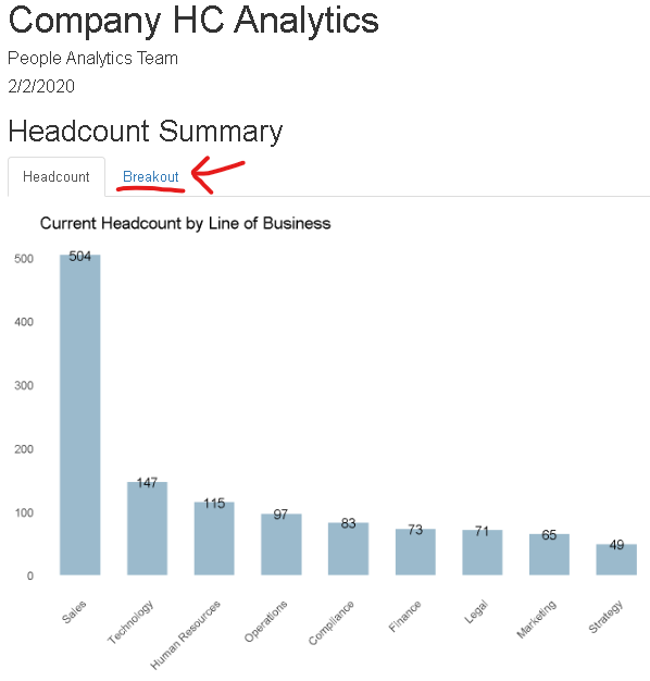
Below is an image of the report we will be building. Note the Headcount tab is currently in focus, showcasing a graph of company headcount. The Breakout tab, marked in red, is hidden.

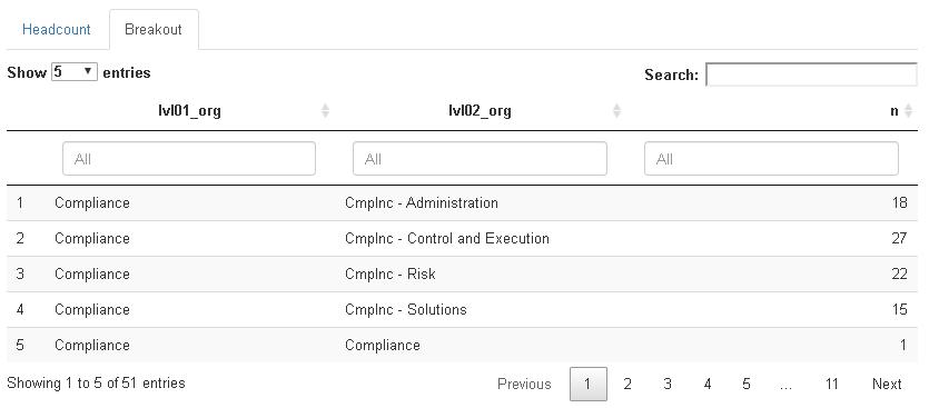
Clicking on the Breakout link takes the user to a second tab containing more detailed headcount data that can be easily searched and filtered:

R Markdown

To create this report, let’s start by opening a new R Markdown document. In RStudio, click File > New File > R Markdown... and click OK. Remove any code on the document and place the setup code below at the top. We’ll use the tidyverse, hrsample, and DT packages.

---
title: "Company HC Analytics"
author: "People Analytics Team"
date: "2/9/2020"
output: html_document
---

```{r setup, include=FALSE}
knitr::opts_chunk$set(echo = TRUE)
library(tidyverse)
library(hrsample) #devtools::install_github("harryahlas/hrsample")
library(DT)
default_color <- rgb(155/255, 186/255, 204/255)
```

Next, let’s add the main header. We’ll also add {.tabset} after the header to designate that the document will have multiple tabs. R will see the ### in front of Headcount and know to make the first tab there.

## Headcount Summary {.tabset}

### Headcount

Now that the first tab is ready to be populated, we can create the data for our graph as well as the graph itself there. Feel free to explore the code that generates the data below. However, for our purposes here you need only copy and paste it to your R Markdown document.

```{r echo=FALSE}
active_roster <- deskhistory_table %>% 
  filter(desk_id_end_date == "2999-01-01") %>% 
  left_join(rollup_view, by = c("desk_id" = "lvl04_desk_id")) %>% 
  left_join(hierarchy_table, by =c("lvl01_desk_id" = "desk_id"))

active_roster %>% 
  count(lvl01_org) %>% 
  filter(lvl01_org != "CEO") %>% 
  ggplot(aes(x = fct_reorder(lvl01_org, -n), y = n)) +
  geom_col(fill = default_color, width = .6) +
  labs(title = "Current Headcount by Line of Business") +
  theme_minimal() +
  theme(panel.grid.major = element_blank(), 
        panel.grid.minor = element_blank(),
        axis.title.y=element_blank(),
        axis.title.x=element_blank(),
        axis.text.x = element_text(angle = 45, hjust = 1)
  ) +
  geom_text(aes(label = n), size = 3.5)
```

Now that we have populated the Headcount tab, we can move on to the Breakout tab. I am amazed at how easy R Markdown makes it to create a new tab.

After we signify the new Breakout tab using ###, we will use the DT package’s datatable function to create a clean table that includes filters and a general text search. The code below generates the table based on data we pulled earlier.

### Breakout
```{r echo=FALSE}
active_roster %>% 
  filter(lvl01_org != "CEO") %>% 
  count(lvl01_org, lvl02_org) %>% 
  datatable(filter = "top", options = list(pageLength = 5))
```

And there you go, the report is ready to knit to HTML. I usually use RStudio’s Knit button but you can do it from the command line as well: rmarkdown::render("your_filename.Rmd", "html_document")

Hope you enjoyed this!

R Markdown

Read more